pytorch 공부 (3) - CNN 구현하기
- 목차
2024.03.08 - [데이터 분석/딥러닝] - pytorch 공부 (2) - ANN 구현하기
CNN 기본
Convolution layer
import torch
import torch.nn as nn

# 합성곱 레이어 객체 생성
layer = nn.Conv2d(1, 20, 5, 1).to(torch.device('cpu')) # 입력 채널 수, 출력 채널 수, 커널 사이즈, stride
layer # Conv2d(1, 20, kernel_size=(5, 5), stride=(1, 1))
- `nn.Conv2d`: Convolution layer. 파라미터는 입력 채널 수, 출력 채널 수, kernel size, stride
- 입력 채널 수, 출력 채널 수는 ANN에서의 사이즈와 같음
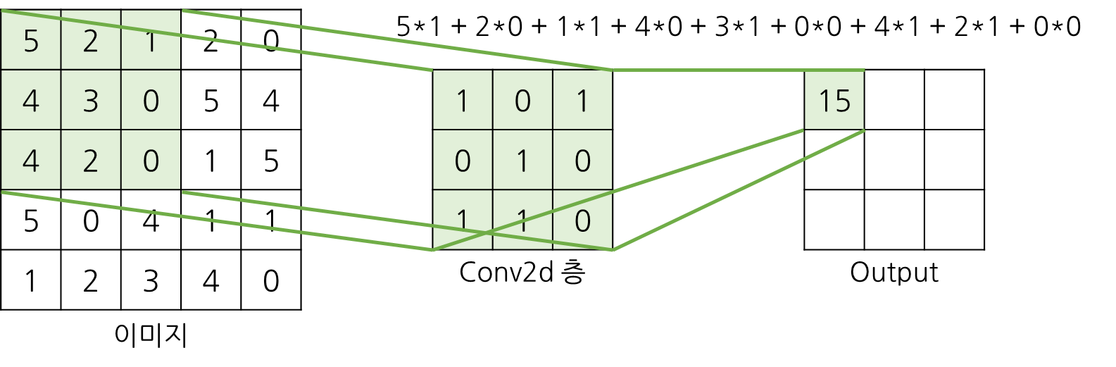
- kernel size: 입력 이미지에 곱해갈 가중치의 크기 (아래 이미지 참고)
- stride: 입력 이미지에 가중치를 곱한 뒤, 다음 스텝으로 갈 때 건너 뛸 픽셀의 수
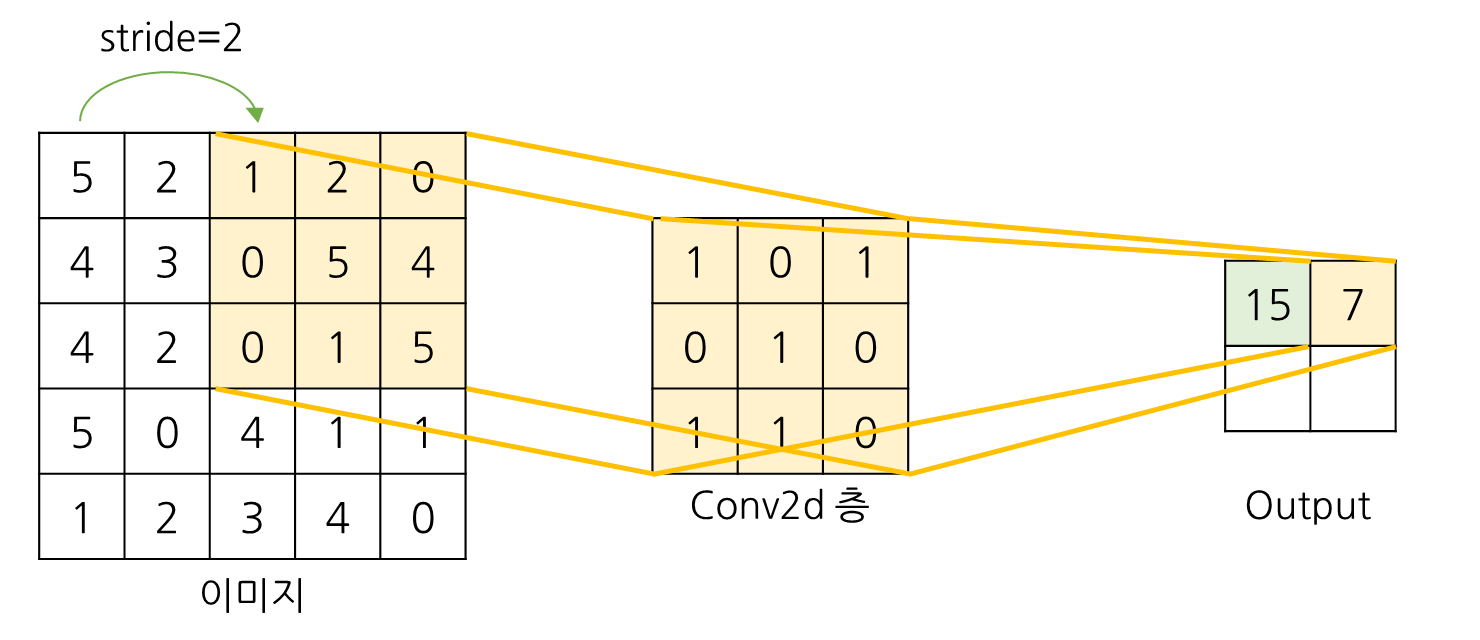
예) 5x5의 이미지를 3x3 kernel, stride가 각각 1과 2인 layer에 통과시킬 경우


가중치 시각화
weight = layer.weight
weight.shape # (20, 1, 5, 5)
import matplotlib.pyplot as plt
plt.imshow(weight[0, 0, :, :], 'gray')
plt.show()
# 입력 이미지와 출력 이미지 비교를 위해 데이터 불러온 후 layer 통과
images, labels = next(iter(train_loader))

output_data = layer(images)
output_data = output_data.data

output = output_data.cpu().numpy()
output.shape # (128, 20, 24, 24)
images.shape # torch.Size([128, 1, 28, 28]) # 5x5 kernel을 통과하여 output이 줄어듬
plt.figure(figsize=(10, 20))
# 원본 이미지
plt.subplot(131)
plt.title('Input')
plt.imshow(images[0, 0, :, :], 'gray')
# 필터 이미지
plt.subplot(132)
plt.title('Weight')
plt.imshow(weight[0, 0, :, :], 'gray')
# 필터 후 이미지
plt.subplot(133)
plt.title('Output')
plt.imshow(output[0, 0, :, :], 'gray')
plt.show()
pooling
# pooling
import torch.nn.functional as f

pool = f.max_pool2d(images, 2, 2) # 커널 사이즈, stride
pool.shape # torch.Size([128, 1, 14, 14])
images.shape # torch.Size([128, 1, 28, 28]) # 커널 사이즈 때문에 크기가 반으로 줄어듬
- `f.max_pool2d`: 이미지(입력), 커널 사이즈, stride인 max pooling layer. max 말고도 mean, min 도 있긴 하지만 잘 안 쓴다.
예) 4x4 이미지를 2x2 kernel, stride=2인 max pooling 층에 통과시킬 경우

이미지의 2x2 사이즈 내 가장 큰 값을 output으로 가져옴
plt.figure(figsize=(10, 15))

# 원본 이미지
plt.subplot(121)
plt.title('Input')
plt.imshow(images[0, 0, :, :], 'gray')

# 풀링 이미지
pool_arr = pool.numpy()

plt.subplot(122)
plt.title('Output')
plt.imshow(pool_arr[0, 0, :, :], 'gray')

plt.show()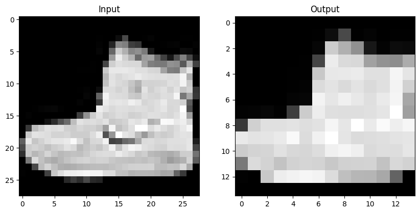
CNN 구현하기
라이브러리 호출 및 디바이스 정의
import torch
import torch.nn as nn
import torch.optim as optim
import torch.nn.functional as f

use_cuda = torch.cuda.is_available()
device = torch.device('cuda' if use_cuda else 'cpu')
CNN 모델 정의
class Cnn(nn.Module):
    def __init__(self):
        super(Cnn, self).__init__()

        self.conv1 = nn.Conv2d(1, 10, 5) # 입력 채널 수=1, 출력 채널 수=10, 커널 사이즈=5, stride=1(기본값)
        self.conv2 = nn.Conv2d(10, 20, 5)
        self.drop = nn.Dropout2d() # 출력값에 Dropout 적용

        # input이 320인 이유는 아래 forward의 주석 확인
        self.fc1 = nn.Linear(320, 160) # 선형결합연산을 수행하는 객체
        self.fc2 = nn.Linear(160, 80) # 히든 레이어
        self.fc3 = nn.Linear(80, 10) # 출력 레이어

    def forward(self, x):
        # 1x28x28 -> 10x24x24 -> 10x12x12
        x = f.relu(f.max_pool2d(self.conv1(x), 2)) # 합성곱 레이어, 풀링, 활성화 함수 순

        # 10x12x12 -> 20x8x8 -> 20x4x4
        x = f.relu(f.max_pool2d(self.drop(self.conv2(x)), 2)) # dropout 추가

        # 20x4x4 -> 1x320
        x = x.view(-1, 320) # 평탄화 작업
        x = f.relu(self.fc1(x))
        x = f.relu(self.fc2(x))
        x = f.dropout(x, training=self.training)
        x = self.fc3(x)
        return x
- `fc1`의 input이 320인 이유
1. 이미지는 1x28x28 데이터 (channel=1이고 가로, 세로가 28인 흑백 데이터)
2. 1x28x28 이미지를 `Conv2d(1, 10, 5)`에 통과시키면 10x24x24 이미지가 된다.
3. 10x24x24 이미지를 `max_pool2d(image, 2)`에 통과시키면 10x12x12 이미지가 된다.
4. 10x12x12 이미지를 `Conv2d(10, 20, 5)`에 통과시키면 20x8x8 이미지가 된다.
5. 20x8x8 이미지를 `max_pool2d(image, 2)`에 통과시키면 20x4x4이미지가 된다.
6. 20x4x4 이미지를 1차원으로 펴면 사이즈가 320인 데이터가 된다.
CNN 모델 학습
model = Cnn().to(device)
optimizer = optim.SGD(model.parameters(), lr=0.01)
EPOCHS = 30
train_history = []
test_history = []
for epoch in range(1, EPOCHS+1):
model.train()
# 학습 데이터를 배치 사이즈만큼 반복
for batch_idx, (data, target) in enumerate(train_loader):
data, target = data.to(device), target.to(device)
optimizer.zero_grad()
output = model(data)
loss = f.cross_entropy(output, target)
loss.backward()
optimizer.step()
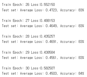
print(f'Train Epoch: {epoch}\tLoss:{loss.item():.6f}')
train_history.append(loss.item())
model.eval() # 검증 모드
test_loss = 0 # 테스트 데이터 오차
correct = 0 # 정답 수
with torch.no_grad(): # 평가 때는 기울기 계산 필요 없음
for data, target in test_loader:
data, target = data.to(device), target.to(device)
output = model(data)
test_loss += f.cross_entropy(output, target, reduction='sum').item()
pred = output.argmax(dim=1, keepdim=True) # dim=1: 차원, keepdim=True: 차원 유지
correct += pred.eq(target.view_as(pred)).sum().item()
test_loss /= len(test_loader.dataset)
test_history.append(test_loss)
print(f'Test set: Average Loss: {test_loss:.4f}, Accuracy: {correct/len(test_loader.dataset)*100:.0f}%\n')- 모델 학습 방법은 ANN과 동일하다.

학습 결과 확인
datas, labels = next(iter(test_loader))

pred = model(datas.to(device))

print('Real:', labels[0].item())
print('Pred:', pred[0].argmax().cpu().item())

"""
Real: 9
Pred: 9
"""
predictions = []
targets = []
with torch.no_grad():
for data, target in test_loader:
data, target = data.to(device), target.to(device)
output = model(data)
pred = output.argmax(dim=1, keepdim=True) # dim=1: 차원, keepdim=True: 차원 유지
pred = pred.detach().cpu().numpy()
target = target.detach().cpu().numpy()
for p, t in zip(pred, target):
predictions.append(p)
targets.append(t)import seaborn as sns
from sklearn.metrics import confusion_matrix
sns.heatmap(confusion_matrix(targets, predictions), annot=True, fmt='d')
plt.xlabel('Pred')
plt.ylabel('Real')
plt.show()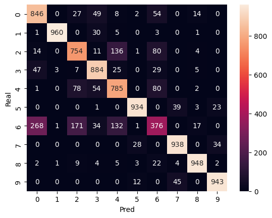
from sklearn.metrics import classification_report

print(classification_report(targets, predictions))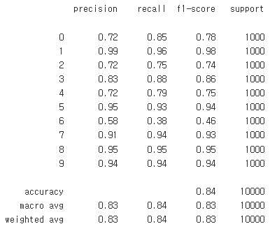
'데이터 분석 > 딥러닝' 카테고리의 다른 글
| torch와 tensorflow를 CNN 코드로 비교하기 (0) | 2024.03.21 |
|---|---|
| pytorch 공부 (3) - RNN 구현하기 (0) | 2024.03.19 |
| torch, tensorflow를 같은 가상환경에 설치하기 (0) | 2024.03.13 |
| pytorch 공부 (2) - ANN 구현하기 (0) | 2024.03.08 |
| pytorch 공부 (1) - 기본 연산 (0) | 2024.03.08 |


